mosmith3asu.github.io
Bio-inspired Passive Power Attenuation Mechanism for Jumping Robot
System Dynamics I
EGR 557 - Group 6
Install Dependencies
!pip install pypoly2tri idealab_tools foldable_robotics pynamics
Requirement already satisfied: pypoly2tri in c:\users\cfc34\miniconda3\envs\fold\lib\site-packages (0.0.3)
Requirement already satisfied: idealab_tools in c:\users\cfc34\miniconda3\envs\fold\lib\site-packages (0.0.22)
Requirement already satisfied: foldable_robotics in c:\users\cfc34\miniconda3\envs\fold\lib\site-packages (0.0.29)
Requirement already satisfied: pynamics in c:\users\cfc34\miniconda3\envs\fold\lib\site-packages (0.0.8)
Requirement already satisfied: numpy in c:\users\cfc34\miniconda3\envs\fold\lib\site-packages (from foldable_robotics) (1.19.2)
Requirement already satisfied: shapely in c:\users\cfc34\miniconda3\envs\fold\lib\site-packages (from foldable_robotics) (1.7.1)
Requirement already satisfied: pyyaml in c:\users\cfc34\miniconda3\envs\fold\lib\site-packages (from foldable_robotics) (5.3.1)
Requirement already satisfied: matplotlib in c:\users\cfc34\miniconda3\envs\fold\lib\site-packages (from foldable_robotics) (3.3.2)
Requirement already satisfied: ezdxf in c:\users\cfc34\miniconda3\envs\fold\lib\site-packages (from foldable_robotics) (0.15)
Requirement already satisfied: imageio in c:\users\cfc34\miniconda3\envs\fold\lib\site-packages (from idealab_tools) (2.9.0)
Requirement already satisfied: scipy in c:\users\cfc34\miniconda3\envs\fold\lib\site-packages (from pynamics) (1.5.2)
Requirement already satisfied: sympy in c:\users\cfc34\miniconda3\envs\fold\lib\site-packages (from pynamics) (1.6.2)
Requirement already satisfied: pyparsing>=2.0.1 in c:\users\cfc34\miniconda3\envs\fold\lib\site-packages (from ezdxf->foldable_robotics) (2.4.7)
Requirement already satisfied: pillow in c:\users\cfc34\miniconda3\envs\fold\lib\site-packages (from imageio->idealab_tools) (8.0.1)
Requirement already satisfied: certifi>=2020.06.20 in c:\users\cfc34\miniconda3\envs\fold\lib\site-packages (from matplotlib->foldable_robotics) (2020.6.20)
Requirement already satisfied: python-dateutil>=2.1 in c:\users\cfc34\miniconda3\envs\fold\lib\site-packages (from matplotlib->foldable_robotics) (2.8.1)
Requirement already satisfied: cycler>=0.10 in c:\users\cfc34\miniconda3\envs\fold\lib\site-packages (from matplotlib->foldable_robotics) (0.10.0)
Requirement already satisfied: kiwisolver>=1.0.1 in c:\users\cfc34\miniconda3\envs\fold\lib\site-packages (from matplotlib->foldable_robotics) (1.3.0)
Requirement already satisfied: six in c:\users\cfc34\miniconda3\envs\fold\lib\site-packages (from cycler>=0.10->matplotlib->foldable_robotics) (1.15.0)
Requirement already satisfied: mpmath>=0.19 in c:\users\cfc34\miniconda3\envs\fold\lib\site-packages (from sympy->pynamics) (1.1.0)


WARNING: You are using pip version 20.3.3; however, version 21.0.1 is available.
You should consider upgrading via the 'c:\users\cfc34\miniconda3\envs\fold\python.exe -m pip install --upgrade pip' command.
Import Packages
%matplotlib inline

import pynamics
from pynamics.frame import Frame
from pynamics.variable_types import Differentiable,Constant
from pynamics.system import System
from pynamics.body import Body
from pynamics.dyadic import Dyadic
from pynamics.output import Output,PointsOutput
from pynamics.particle import Particle
import pynamics.integration
from math import pi
import numpy as np
import matplotlib.pyplot as plt
from matplotlib import animation, rc
from IPython.display import HTML
plt.ion()
Assignment
1. Scale
Ensure your system is using SI units. You should be specifying lengths in meters (so millimeters should be scaled down to the .001 range), forces in Newtons, and radians (not degrees), and masses in kg. You may make educated guesses about mass for now.
Since our system is relatively small and the jumping and landing happens quickly, the units of the dynamics have to be scaled to avoid numerical error that can cause the solver to diverge. In the literature[1], the takeoff of jumping happens over only about 30 milisecond. The unit used is centimeter for length, gram for weight, and 0.01 second for time. The unit of other derived values are scaled accordingly.
# Unit scaling
M_TO_L = 1e2 # cm
KG_TO_W = 1e3 # 1g
S_TO_T = 1e2 # 0.01s

# Integration tolerance
tol = 1e-4

# Time parameters
tinitial = 0
tfinal = 0.1*S_TO_T
fps = 30
tstep = 1/fps
t = np.r_[tinitial:tfinal:tstep]
# Define system
system = System()
pynamics.set_system(__name__,system)
# Impact force properties
impactV = 3.1*M_TO_L/S_TO_T # m/s
payloadMass = 0.097*KG_TO_W # kg
gravity = 9.81*M_TO_L/S_TO_T**2 # m/s^2

# System constants
g = Constant(gravity,'g',system)
b = Constant(0*KG_TO_W*M_TO_L**2/S_TO_T,'b',system) # global joint damping, (kg*(m/s^2)*m)/(rad/s)
bQ = Constant(0*KG_TO_W*M_TO_L**2/S_TO_T,'bQ',system) # tendon joint damping, (kg*(m/s^2)*m)/(rad/s)
kQ = Constant(0.08*KG_TO_W*M_TO_L**2/S_TO_T**2,'kQ',system) # tendon joint spring, (kg*m/s^2*m)/(rad)
load = Constant(1*KG_TO_W*M_TO_L/S_TO_T**2,'load',system) # load at toe, kg*m/s^2
# Link lengths (m)
len_n = 0.015*M_TO_L
len_a1 = 0.010*M_TO_L
len_a2 = 0.017*M_TO_L
len_b = 0.010*M_TO_L
len_c = 0.020*M_TO_L
len_d1 = 0.020*M_TO_L
len_d2 = 0.025*M_TO_L
len_e = 0.046*M_TO_L
len_f = 0.010*M_TO_L
len_g1 = 0.010*M_TO_L
len_g2 = 0.032*M_TO_L

# Link length constants
lN = Constant(len_n,'lN',system)
lA1 = Constant(len_a1,'lA1',system)
lA2 = Constant(len_a2,'lA2',system)
lB = Constant(len_b,'lB',system)
lC = Constant(len_c,'lC',system)
lD1 = Constant(len_d1,'lD1',system)
lD2 = Constant(len_d2,'lD2',system)
lE = Constant(len_e,'lE',system)
lF = Constant(len_f,'lF',system)
lG1 = Constant(len_g1,'lG1',system)
lG2 = Constant(len_g2,'lG2',system)
# Beam properties
beam_density = 689*KG_TO_W/M_TO_L**3 # kg/m^3 - cardboard
beam_thickness = 0.00025*M_TO_L # m
beam_width = 0.020*M_TO_L # m
kgpm = beam_density * beam_thickness * beam_width # kg per meter

# Masses (kg)
mA = Constant((len_a1+len_a2)*kgpm,'mA',system)
mB = Constant(len_b*kgpm,'mB',system)
mC = Constant(len_c*kgpm,'mC',system)
mD = Constant((len_d1+len_d2)*kgpm,'mD',system)
mE = Constant(len_e*kgpm,'mE',system)
mF = Constant(len_f*kgpm,'mF',system)
mG = Constant((len_g1+len_g2)*kgpm,'mG',system)
2. Define Inertias
Add a center of mass and a particle or rigid body to each rotational frame. You may use particles for now if you are not sure of the inertial properties of your bodies, but you should plan on finding these values soon for any “payloads” or parts of your system that carry extra loads (other than the weight of paper).
# Inertias calculated based on a rectangular prism and uniform density
Ixx_A = Constant((1/12)*(len_a1+len_a2)*kgpm*(beam_width**2 + beam_thickness**2), 'Ixx_A', system)
Iyy_A = Constant((1/12)*(len_a1+len_a2)*kgpm*((len_a1+len_a2)**2 + beam_width**2), 'Iyy_A', system)
Izz_A = Constant((1/12)*(len_a1+len_a2)*kgpm*((len_a1+len_a2)**2 + beam_thickness**2),'Izz_A',system)

Ixx_B = Constant((1/12)*len_b*kgpm*(beam_width**2 + beam_thickness**2), 'Ixx_B', system)
Iyy_B = Constant((1/12)*len_b*kgpm*(len_b**2 + beam_width**2), 'Iyy_B', system)
Izz_B = Constant((1/12)*len_b*kgpm*(len_b**2 + beam_thickness**2),'Izz_B',system)

Ixx_C = Constant((1/12)*len_c*kgpm*(beam_width**2 + beam_thickness**2), 'Ixx_C', system)
Iyy_C = Constant((1/12)*len_c*kgpm*(len_c**2 + beam_width**2), 'Iyy_C', system)
Izz_C = Constant((1/12)*len_c*kgpm*(len_c**2 + beam_thickness**2),'Izz_C',system)

Ixx_D = Constant((1/12)*(len_d1+len_d2)*kgpm*(beam_width**2 + beam_thickness**2), 'Ixx_D', system)
Iyy_D = Constant((1/12)*(len_d1+len_d2)*kgpm*((len_d1+len_d2)**2 + beam_width**2), 'Iyy_D', system)
Izz_D = Constant((1/12)*(len_d1+len_d2)*kgpm*((len_d1+len_d2)**2 + beam_thickness**2),'Izz_D',system)

Ixx_E = Constant((1/12)*len_e*kgpm*(beam_width**2 + beam_thickness**2), 'Ixx_E', system)
Iyy_E = Constant((1/12)*len_e*kgpm*(len_e**2 + beam_width**2), 'Iyy_E', system)
Izz_E = Constant((1/12)*len_e*kgpm*(len_e**2 + beam_thickness**2),'Izz_E',system)

Ixx_F = Constant((1/12)*len_f*kgpm*(beam_width**2 + beam_thickness**2), 'Ixx_F', system)
Iyy_F = Constant((1/12)*len_f*kgpm*(len_f**2 + beam_width**2), 'Iyy_F', system)
Izz_F = Constant((1/12)*len_f*kgpm*(len_f**2 + beam_thickness**2),'Izz_F',system)

Ixx_G = Constant((1/12)*(len_g1+len_g2)*kgpm*(beam_width**2 + beam_thickness**2), 'Ixx_G', system)
Iyy_G = Constant((1/12)*(len_g1+len_g2)*kgpm*((len_g1+len_g2)**2 + beam_width**2), 'Iyy_G', system)
Izz_G = Constant((1/12)*(len_g1+len_g2)*kgpm*((len_g1+len_g2)**2 + beam_thickness**2),'Izz_G',system)
# State variables
qA,qA_d,qA_dd = Differentiable('qA',system)
qB,qB_d,qB_dd = Differentiable('qB',system)
qC,qC_d,qC_dd = Differentiable('qC',system)
qD,qD_d,qD_dd = Differentiable('qD',system)
qE,qE_d,qE_dd = Differentiable('qE',system)
qF,qF_d,qF_dd = Differentiable('qF',system)
qG,qG_d,qG_dd = Differentiable('qG',system)

statevariables = system.get_state_variables()
# Initial values for state variables (taken from numeric solution)
initialvalues = {}
initialvalues[qA] = -0.43633231
initialvalues[qA_d] = 0
initialvalues[qB] = -2.35619449
initialvalues[qB_d] = 0
initialvalues[qC] = 1.77374098
initialvalues[qC_d] = 0
initialvalues[qD] = -1.94056282
initialvalues[qD_d] = 0
initialvalues[qE] = -1.88232585
initialvalues[qE_d] = 0
initialvalues[qF] = 1.57079633
initialvalues[qF_d] = 0
initialvalues[qG] = 0.54939865
initialvalues[qG_d] = 0
ini = [initialvalues[item] for item in statevariables]
# Frames
N = Frame('N')
A = Frame('A')
B = Frame('B')
C = Frame('C')
D = Frame('D')
E = Frame('E')
F = Frame('F')
G = Frame('G')
system.set_newtonian(N)

# Rotate frames
A.rotate_fixed_axis_directed(N,[0,0,1],qA,system)
B.rotate_fixed_axis_directed(N,[0,0,1],qB,system)
C.rotate_fixed_axis_directed(B,[0,0,1],qC,system)
D.rotate_fixed_axis_directed(A,[0,0,1],qD,system)
E.rotate_fixed_axis_directed(A,[0,0,1],qE,system)
F.rotate_fixed_axis_directed(D,[0,0,1],qF,system)
G.rotate_fixed_axis_directed(F,[0,0,1],qG,system)
# Kinematics
pNA = 0*N.x
pNB = -lN*N.x
pBC = pNB + lB*B.x
pAD = pNA + lA1*A.x
pCD = pBC + lC*C.x
pCD_p = pAD + lD1*D.x
pAE = pNA + (lA1+lA2)*A.x
pDF= pAD + (lD1+lD2)*D.x
pFG = pDF + lF*F.x
pEG = pFG + lG1*G.x
pEG_p = pAE + lE*E.x
pNH = pFG + (lG1+lG2)*G.x # Toe
# Centers of mass
pAcm = pNA + ((lA1+lA2)/2)*A.x
pBcm = pNB + (lB/2)*B.x
pCcm = pBC + (lC/2)*C.x
pDcm = pAD + ((lD1+lD2)/2)*D.x
pEcm = pAE + (lE/2)*E.x
pFcm = pDF + (lF/2)*F.x
pGcm = pFG + ((lG1+lG2)/2)*G.x
# Toe velocity
vNH = pNH.time_derivative(N, system)

# Joint angular velocities
wA = N.getw_(A)
wB = N.getw_(B)
wC = N.getw_(C)
wD = N.getw_(D)
wE = N.getw_(E)
wF = N.getw_(F)
wG = N.getw_(G)
# Bodies
IA = Dyadic.build(A,Ixx_A,Iyy_A,Izz_A)
IB = Dyadic.build(B,Ixx_B,Iyy_B,Izz_B)
IC = Dyadic.build(C,Ixx_C,Iyy_C,Izz_C)
ID = Dyadic.build(D,Ixx_D,Iyy_D,Izz_D)
IE = Dyadic.build(E,Ixx_E,Iyy_E,Izz_E)
IF = Dyadic.build(F,Ixx_F,Iyy_F,Izz_F)
IG = Dyadic.build(G,Ixx_G,Iyy_G,Izz_G)

BodyA = Body('BodyA',A,pAcm,mA,IA,system)
BodyB = Body('BodyB',B,pBcm,mB,IB,system)
BodyC = Body('BodyC',C,pCcm,mC,IC,system)
BodyD = Body('BodyD',D,pDcm,mD,ID,system)
BodyE = Body('BodyE',E,pEcm,mE,IE,system)
BodyF = Body('BodyF',F,pFcm,mF,IF,system)
BodyG = Body('BodyG',G,pGcm,mG,IG,system)
3. Add Forces
Add the acceleration due to gravity. Add rotational springs in the joints (using k=0 is ok for now) and a damper to at least one rotational joint. You do not need to add external motor/spring forces but you should start planning to collect that data.
# Load forces
system.addforce(load*N.y, vNH)

# Spring joint
system.add_spring_force1(kQ, (qG - initialvalues[qG])*N.z, wG)
system.addforce(-bQ*wG, wG)

# Dampers on angular velocities
system.addforce(-b*wA, wA)
system.addforce(-b*wB, wB)
system.addforce(-b*wC, wC)
system.addforce(-b*wD, wD)
system.addforce(-b*wE, wE)
system.addforce(-b*wF, wF)

# Gravity
system.addforcegravity(-g*N.y)
4. Constraints
Keep mechanism constraints in, but follow the pendulum example of double-differentiating all constraint equations.
# Constraints
eq = [
      # Lock point CD in place
    (pCD-pCD_p).dot(N.x), # pCD can only move in the along the base frame x-axis
    (pCD-pCD_p).dot(N.y), # pCD can only move in the along the base frame y-axis
    # Lock point EG in place
    (pEG-pEG_p).dot(N.x), # pEG can only move in the along the base frame x-axis
    (pEG-pEG_p).dot(N.y), # pEG can only move in the along the base frame y-axis
    qA - initialvalues[qA], # joint A does not rotate
    qB - initialvalues[qB], # joint B does not rotate
]

eq_d=[(system.derivative(item)) for item in eq]
eq_dd=[(system.derivative(item)) for item in eq_d]
5. Solution
Add the code from the bottom of the pendulum example for solving for f=ma, integrating, plotting, and animating. Run the code to see your results. It should look similar to the pendulum example with constraints added, as in like a rag-doll or floppy
# F=ma
f,ma = system.getdynamics()
2021-02-28 22:47:50,308 - pynamics.system - INFO - getting dynamic equations
# Solve for acceleration
func1,lambda1 = system.state_space_post_invert(f,ma,eq_dd,return_lambda = True)
2021-02-28 22:47:51,052 - pynamics.system - INFO - solving a = f/m and creating function
2021-02-28 22:47:51,063 - pynamics.system - INFO - substituting constrained in Ma-f.
2021-02-28 22:47:52,880 - pynamics.system - INFO - done solving a = f/m and creating function
2021-02-28 22:47:52,881 - pynamics.system - INFO - calculating function for lambdas
# Integrate
states=pynamics.integration.integrate(func1,ini,t,rtol=tol,atol=tol, args=({'constants':system.constant_values},))
2021-02-28 22:47:53,087 - pynamics.integration - INFO - beginning integration
2021-02-28 22:47:53,088 - pynamics.system - INFO - integration at time 0000.00
2021-02-28 22:47:55,607 - pynamics.system - INFO - integration at time 0006.70
2021-02-28 22:47:56,832 - pynamics.integration - INFO - finished integration
# Outputs
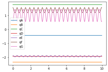
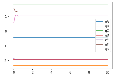
plt.figure()
artists = plt.plot(t,states[:,:7])
plt.legend(artists,['qA','qB','qC','qD','eE','qF','qG'])
<matplotlib.legend.Legend at 0x1890e0e7220>
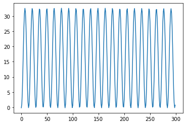
# Energy
KE = system.get_KE()
PE = system.getPEGravity(pNA) - system.getPESprings()
energy_output = Output([KE-PE],system)
energy_output.calc(states)
energy_output.plot_time()
2021-02-28 22:47:57,183 - pynamics.output - INFO - calculating outputs
2021-02-28 22:47:57,213 - pynamics.output - INFO - done calculating outputs
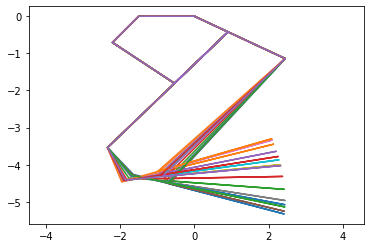
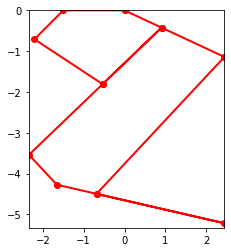
# Motion
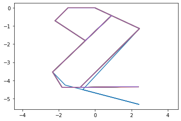
points = [pNA,pNB,pBC,pCD,pDF,pFG,pEG,pNH,pEG,pAE,pAD,pCD,pAD,pNA]
points_output = PointsOutput(points,system)
y = points_output.calc(states)
points_output.plot_time(20)
2021-02-28 22:47:57,425 - pynamics.output - INFO - calculating outputs
2021-02-28 22:47:57,494 - pynamics.output - INFO - done calculating outputs


<AxesSubplot:>
# Animate
points_output.animate(fps = fps,movie_name = 'without-damping.mp4',lw=2,marker='o',color=(1,0,0,1),linestyle='-')
<AxesSubplot:>
# Animate in Jupyter
HTML(points_output.anim.to_html5_video())
With a damping value of zero, the current system oscillates due to the elastics in the system. The motion seen in the video occurs over 100ms.
6. Tuning
Now adjust the damper value to something nonzero, that over 10s shows that the system is settling.
# System constants
g = Constant(gravity,'g',system)
b = Constant(0*KG_TO_W*M_TO_L**2/S_TO_T,'b',system) # global joint damping, (kg*(m/s^2)*m)/(rad/s)
bQ = Constant(0.0001*KG_TO_W*M_TO_L**2/S_TO_T,'bQ',system) # tendon joint damping, (kg*(m/s^2)*m)/(rad/s)
kQ = Constant(0.08*KG_TO_W*M_TO_L**2/S_TO_T**2,'kQ',system) # tendon joint spring, (kg*m/s^2*m)/(rad)
load = Constant(1*KG_TO_W*M_TO_L/S_TO_T**2,'load',system) # load at toe, kg*m/s^2
# F=ma
f,ma = system.getdynamics()
2021-02-28 22:48:17,818 - pynamics.system - INFO - getting dynamic equations
# Solve for acceleration
func1,lambda1 = system.state_space_post_invert(f,ma,eq_dd,return_lambda = True)
2021-02-28 22:48:18,556 - pynamics.system - INFO - solving a = f/m and creating function
2021-02-28 22:48:18,565 - pynamics.system - INFO - substituting constrained in Ma-f.
2021-02-28 22:48:20,096 - pynamics.system - INFO - done solving a = f/m and creating function
2021-02-28 22:48:20,097 - pynamics.system - INFO - calculating function for lambdas
# Integrate
states=pynamics.integration.integrate(func1,ini,t,rtol=tol,atol=tol, args=({'constants':system.constant_values},))
2021-02-28 22:48:20,117 - pynamics.integration - INFO - beginning integration
2021-02-28 22:48:20,118 - pynamics.system - INFO - integration at time 0000.00
2021-02-28 22:48:20,702 - pynamics.integration - INFO - finished integration
# Outputs
plt.figure()
artists = plt.plot(t,states[:,:7])
plt.legend(artists,['qA','qB','qC','qD','eE','qF','qG'])
<matplotlib.legend.Legend at 0x1890fef25b0>
# Energy
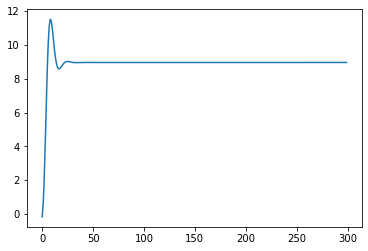
KE = system.get_KE()
PE = system.getPEGravity(pNA) - system.getPESprings()
energy_output = Output([KE-PE],system)
energy_output.calc(states)
energy_output.plot_time()
2021-02-28 22:48:21,041 - pynamics.output - INFO - calculating outputs
2021-02-28 22:48:21,072 - pynamics.output - INFO - done calculating outputs
# Motion
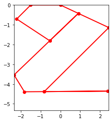
points = [pNA,pNB,pBC,pCD,pDF,pFG,pEG,pNH,pEG,pAE,pAD,pCD,pAD,pNA]
points_output = PointsOutput(points,system)
y = points_output.calc(states)
points_output.plot_time(20)
2021-02-28 22:48:21,255 - pynamics.output - INFO - calculating outputs
2021-02-28 22:48:21,321 - pynamics.output - INFO - done calculating outputs


<AxesSubplot:>
# Animate
points_output.animate(fps = fps,movie_name = 'with-damping.mp4',lw=2,marker='o',color=(1,0,0,1),linestyle='-')
<AxesSubplot:>
# Animate in Jupyter
HTML(points_output.anim.to_html5_video())
With damping added to the system, the linkages come to rest approximately 0.01 second(out of the entire 0.1 sceond) after the force is applied. The system remains in equilibirum for the remaining time.
Refernces
[1] M. J. Schwaner, D. C. Lin, and C. P. McGowan, “Jumping mechanics of desert kangaroo rats,” Journal of Experimental Biology, vol. 221, no. 22, 2018, doi: 10.1242/jeb.186700.